I am curious as to how such a network would perform with a non-linear output activation function, say tanh since it seems to work well. I am asking because the neutrals are still not quite right - perhaps because L is not linear (identity)?
As far as I know, the preferred output activation function (this is the function used in the last layer, the one that provides the output values; L, a and b in our case) for numerical regression is the identity. In other words, it is the rest of the network which is in charge of modelling the non-linearities, the output layer just performs a linear combination over its inputs. Non-linear output activation functions (like sigmoid or tanh) are preferred for logistic regression problems (i.e. classification problems). But I can do a quick test using sigmoid and tanh in the output layer.
For completeness the linear 3x3 matrix fit to the V3 reference spectro measurements results in the following:
dE76 mean = 3.569, dE76 median = 2.461, dE76 max = 21.709
That is clearly better, but in the same order of magnitude as the linear NN (MLP_XYZ_()).
With a fairly simple NN (MLP_XYZ_(3, 3)_tanh_identity) the NN beats the optimum linear fit.
MLP_XYZ_()_tanh_identity : ΔE_max = 33.6562 , ΔE_mean = 3.2097 , ΔE_median = 1.8020
MLP_XYZ_(3, 3)_tanh_identity : ΔE_max = 15.3840 , ΔE_mean = 2.4645 , ΔE_median = 1.8418
MLP_XYZ_(4, 4)_tanh_identity : ΔE_max = 11.2728 , ΔE_mean = 2.0082 , ΔE_median = 1.5386
What we might be seeing is a combination of overfitting and the inability of the NN to properly represent the Lab gamma curve.
1. Overfitting
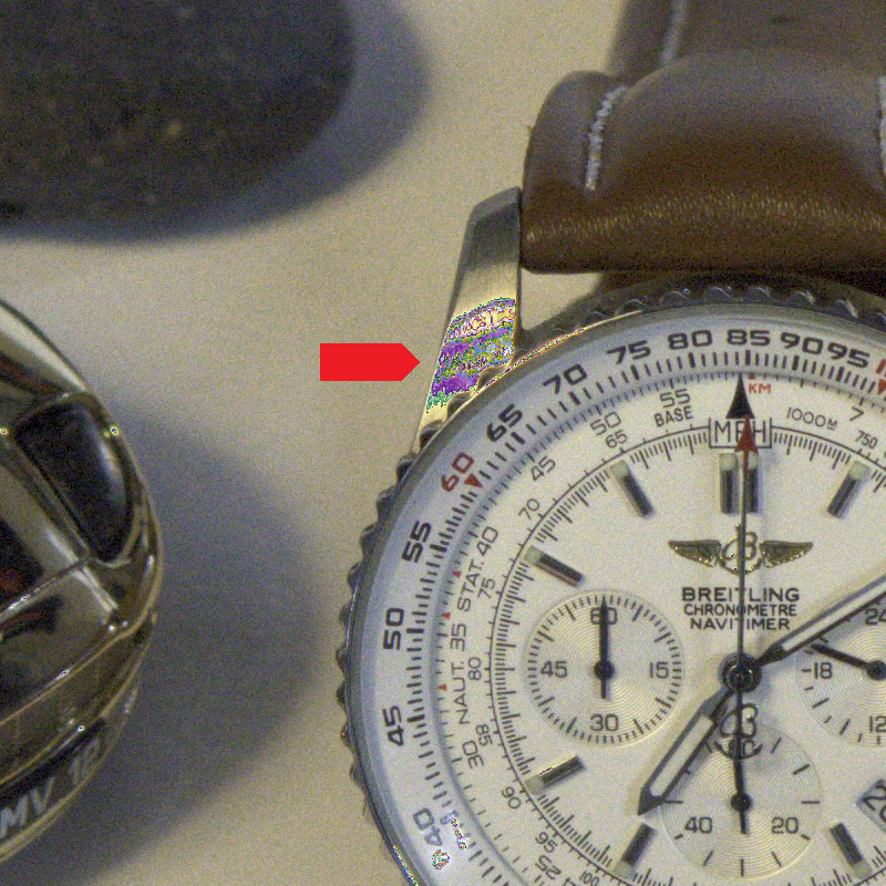
If you look at the attached annotation on your L graph, you can see we have outliers (the arrows) but not what seems as random deviation.
2. Gamma curve
In the same attachment in the circle you can see something that looks like ringing. I suspect that this is a result of an inability to properly represent Lab gamma. The tanh activation curve looks somewhat like the gamma curve, but isn't. (Nor is it a linear transition in case of XYZ).
Now, in my never humble opinion I would assess the results as follows:
(50, 50) allows too much variation in curves and fitting. There are several reasons you should NOT want to make the layers that large. One vitally important reason is that NN is supposed to encode patterns compactly that are either too large for us to comprehend or too hard for us to understand, or both. By applying large NN layers for what is essentially a really simple linear matrix conversion, we are not making the solution elegantly small and succinct.
So, in this case I would ask myself what would be necessary for the NN to better match the gamma curve (or the linear curve) which I suspect will better match the overall model without overfitting? Keeping it elegantly small?
My answer would be: add another hidden layer. The NN probably just needs another step for better matching the gamma curves. And, to keep it as small as possible, I would first try (4, 4, 4) and then if it confirms the suspicion, reduce to (4, 4, 3), (3, 4, 3), and maybe (3, 3, 3).
That's very interesting insights, will give them a try. But with deep NN like (200,200,200) the improvement was none, so surely the complexity of the NN was far beyond the complexity of the problem.
What we might be having here is just an innacurate gamma curve fitting in the low end, and the undesired overfitting maybe cause by 'noise': samples having less accuracy because of noise and influence of undesired reflections in the IT8 capture. If we look at the somewhat gamma-like curve I plotted in my previous post (output L values vs input RAW_WB G), the curve doesn't converge softly to (G=0, L=0), and it should. Instead, low G values correspond to even lower than expected L values so the NN seems to be clipping the shadows. This makes me think the RAW file in the dark shadows could be contaminated by some degree of reflection on the chart. A possible solution would be to drop the darkest patches in the training set they are not respecting the sensor linear response), and synthetically introduce (R=0, G=0, B=0) -> (L=0, a=0, b=0) examples in the training set, because we really need L=0 in absence of light, but not before that.
A similar kind of issue may be taking place in the highlights: the NN has not been trained with a (R=255, G=255, B=255) -> (L=100, a=0, b=0) example, nor with partial saturations (some channel clipped while the others are fine). This may explain this undesired behaviour in partially clipped highlights (this is the NN RAW RGB_WB to Lab output, later to ProPhotoRGB):
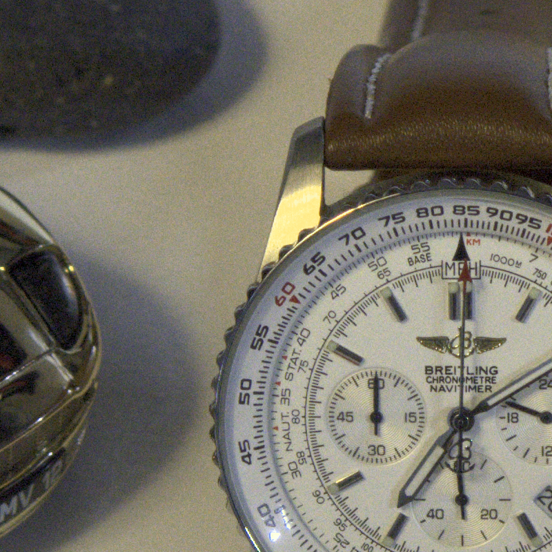
Just using input values with -0.5EV exposure, the problem is not there:
Anyway I think this is a more complex to fix problem than the low end one, and solving all possible cases of clipped highlights is out of the scope of the exercise. In fact RAW developers need to implement complex highlight strategies to deal with this problem.
---
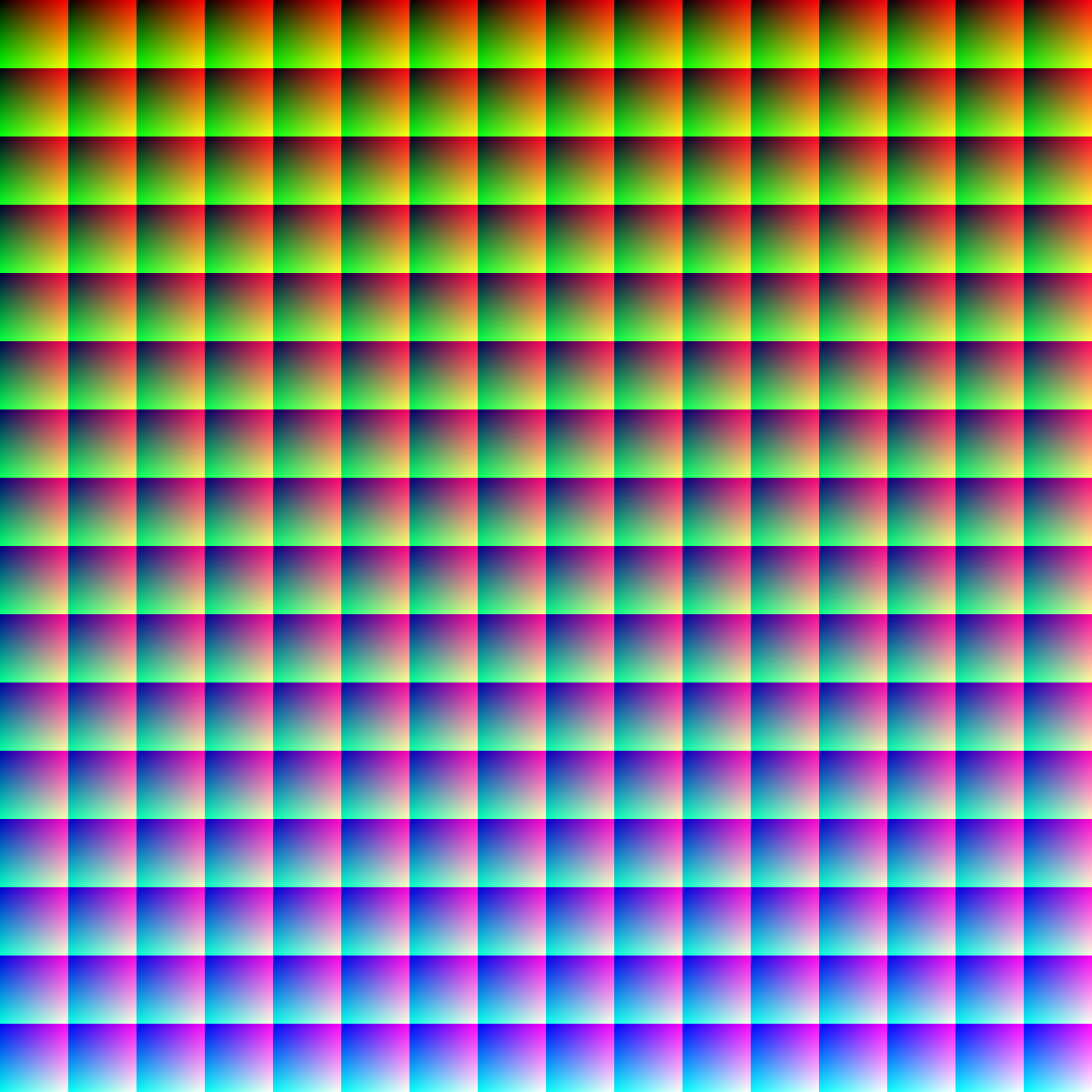
Before doing more simulations or picking some patch pairs to predict the interpolated colours between them, I did a brute force exercise feeding the NN with all possible RGB 8-bit combinations in a synthetic image by Bruce Lindbloom, which shows smooth gradients:
After being transformed by the NN, we get again smooth gradients in the output what makes me think again that the NN is not oscillating because of overftting when predicting in-between colours:
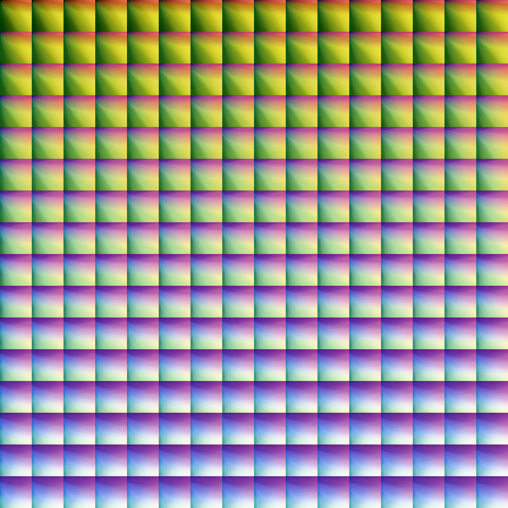
Maybe I'm oversimplifying my conclusions here, but if the NN would be generating unstable outputs for unseen colours, I think we should see that behaviour here, do you agree?.
Regards
